The schedule is out 🗓️ for POSETTE: An Event for Postgres 2026!
Everybody counts, but not always quickly. This article is a close look into how PostgreSQL optimizes counting. If you know the tricks there are ways to count rows orders of magnitude faster than you do already.
The problem is actually underdescribed—there are several variations of counting, each with its own methods. First think whether you need an exact count or whether an estimate suffices. Next, are you counting duplicates or just distinct values? Finally do you want a lump count of an entire table or will you want to count only those rows matching extra criteria?
We'll analyze the techniques available for each situation and compare their speed and resource consumption. After learning about techniques for a single database we'll use Citus to demonstrate how to parallelize counts in a distributed database.
Table of Contents
- Preparing the DB for tests
- Counts With Duplicates
- Distinct Counts (No Duplicates)
- Parallelization
- Reference of Techniques
Preparing the DB for tests
The sections below use the following table for benchmarks.
-- create a million random numbers and strings
CREATE TABLE items AS
  SELECT
    (random()*1000000)::integer AS n,
    md5(random()::text) AS s
  FROM
    generate_series(1,1000000);

-- inform planner of big table size change
VACUUM ANALYZE;
Counts With Duplicates
Exact Counts
Let's begin at the beginning, exact counts allowing duplication over some or all of a table, good old count(*). Measuring the time to run this command provides a basis for evaluating the speed of other types of counting.
Pgbench provides a convenient way to run a query repeatedly and collect statistics about performance.
# Tests in this article were run against PostgreSQL 9.5.4

echo "SELECT count(*) FROM items;" | pgbench -d count -t 50 -P 1 -f -

# average  84.915 ms
# stddev    5.251 ms
A note about count(1) vs count(*). One might think that count(1) would be faster because count(*) appears to consult the data for a whole row. However the opposite is true. The star symbol is meaningless here, unlike its use in SELECT *. PostgreSQL parses The expression count(*) as a special case taking no arguments. (Historically the expression ought to have been defined as count().) On the other hand count(1) takes an argument and PostgreSQL has to check at every row to see that ts argument, 1, is indeed still not NULL.
Running the above benchmark with count(1) results in:
# average  98.896 ms
# stddev    7.280 ms
However both both forms of count(1) and count(*) are fundamentally slow. PostgreSQL uses multiversion concurrency control (MVCC) to ensure consistency between simultaneous transactions. This means each transaction may see different rows -- and different numbers of rows -- in a table. There is no single universal row count that the database could cache, so it must scan through all rows counting how many are visible. Performance for an exact count grows linearly with table size.
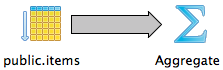
EXPLAIN SELECT count(*) FROM items;

Aggregate  (cost=20834.00..20834.01 rows=1 width=0)
  ->  Seq Scan on items  (cost=0.00..18334.00 rows=1000000 width=0)
The scan accounts for 88% of the total cost. As we double the table size the query time roughly doubles, with cost of scanning and aggregating growing proportionally with one other.
| Rows | Avg Time |
|---|---|
| 1M | 85ms |
| 2M | 161ms |
| 4M | 343ms |
How can we make this faster? Something has to give, either we can settle for an estimated rather than exact count, or we can cache the count ourselves using a manual increasing-decreasing tally. However in the second case we have to keep a tally for each table and where clause that we want to count quickly later.
Here's an example of the tally approach applied to the whole items table. The following trigger-based solution is adapted from A. Elein Mustain. PostgreSQL's MVCC will maintain consistency between the items table and a table of row counts.
BEGIN;

CREATE TABLE row_counts (
  relname   text PRIMARY KEY,
  reltuples bigint
);

-- establish initial count
INSERT INTO row_counts (relname, reltuples)
  VALUES ('items', (SELECT count(*) from items));

CREATE OR REPLACE FUNCTION adjust_count()
RETURNS TRIGGER AS
$$
   DECLARE
   BEGIN
   IF TG_OP = 'INSERT' THEN
      EXECUTE 'UPDATE row_counts set reltuples=reltuples +1 where relname = ''' || TG_RELNAME || '''';
      RETURN NEW;
   ELSIF TG_OP = 'DELETE' THEN
      EXECUTE 'UPDATE row_counts set reltuples=reltuples -1 where relname = ''' || TG_RELNAME || '''';
      RETURN OLD;
   END IF;
   END;
$$
LANGUAGE 'plpgsql';

CREATE TRIGGER items_count BEFORE INSERT OR DELETE ON items
  FOR EACH ROW EXECUTE PROCEDURE adjust_count();

COMMIT;
The speed of reading and updating the cached value is independent of the table size, and reading is very fast. However this technique shifts overhead to inserts and deletes. Without the trigger the following statement takes an average of 4.7 seconds, whereas inserts with the trigger are fifty times slower:
INSERT INTO items (n, s)
  SELECT
    (random()*1000000)::integer AS n,
    md5(random()::text) AS s
  FROM generate_series(1,1000000);
Estimated Counts
Full Table Estimates
The previous "tally" approach for caching table counts makes inserts slow. If we're willing to accept an estimated rather than exact count we can get fast reads like the tally but with no insert degradation. To do so we can lean on estimates gathered from PostgreSQL subsystems. Two sources are the stats collector and the autovacuum daemon.
Here are two alternatives for getting the estimate:
-- Asking the stats collector
SELECT n_live_tup
  FROM pg_stat_all_tables
 WHERE relname = 'items';

-- Updated by VACUUM and ANALYZE
SELECT reltuples
  FROM pg_class
 WHERE relname = 'items';
However there's a more accurate source that is less likely to be stale. Andrew Gierth (RhodiumToad) advises:
Remember that reltuples isn't the estimate that the planner actually uses; the planner uses reltuples/relpages multiplied by the current number of pages.
Here's the intuition. As the sample of data in a table increases then the average number of rows fitting in a physical page is likely to change less drastically than number of rows total. We can multiply the average rows per page by up-to-date information about the current number of pages occupied by a table for a more accurate estimation of the current number of rows.
-- pg_relation_size and block size have fresh info so combine them with
-- the estimation of tuples per page
SELECT
  (reltuples/relpages) * (
    pg_relation_size('items') /
    (current_setting('block_size')::integer)
  )
  FROM pg_class where relname = 'items';
Filtered Table Estimates
The previous section gets estimated counts for entire tables, but is there a way to get one for only those rows matching a condition? Michael Fuhr came up with a clever trick to run EXPLAIN for a query and parse its output.
CREATE FUNCTION count_estimate(query text) RETURNS integer AS $$
DECLARE
  rec   record;
  rows  integer;
BEGIN
  FOR rec IN EXECUTE 'EXPLAIN ' || query LOOP
    rows := substring(rec."QUERY PLAN" FROM ' rows=([[:digit:]]+)');
    EXIT WHEN rows IS NOT NULL;
  END LOOP;
  RETURN rows;
END;
$$ LANGUAGE plpgsql VOLATILE STRICT;
We can use the function like this:
SELECT count_estimate('SELECT 1 FROM items WHERE n < 1000');
The accuracy of this method relies on the planner which uses several techniques to estimate the selectivity of a where clause and from there the number of rows that will be returned.
Distinct Counts (No Duplicates)
Exact Counts
Default behavior under low memory
Count with duplicates may be slow, but count distinct is much worse. With limited working memory and no indices, PostgreSQL is unable to optimize much. In its stock configuration PostgreSQL specifies a low memory limit per concurrent query (work_mem). On my development machine the default was four megabytes.
Sticking with default, here is the performance for dealing with a million rows.
echo "SELECT count(DISTINCT n) FROM items;" | pgbench -d count -t 50 -P 1 -f -
# average  742.855 ms
# stddev    21.907 ms
echo "SELECT count(DISTINCT s) FROM items;" | pgbench -d count -t 5 -P 1 -f -
# average  31747.337 ms
# stddev     267.183 ms
Running EXPLAIN shows that the bulk of the query happens in the aggregate, and that running the count on a string column takes longer than the integer column:
-- plan for the integer column, n
Aggregate  (cost=20834.00..20834.01 rows=1 width=4) (actual time=860.620..860.620 rows=1 loops=1)
  Output: count(DISTINCT n)
  Buffers: shared hit=3904 read=4430, temp read=1467 written=1467
  ->  Seq Scan on public.items  (cost=0.00..18334.00 rows=1000000 width=4) (actual time=0.005..107.702 rows=1000000 loops=1)
        Output: n, s
        Buffers: shared hit=3904 read=4430

-- plan for the text column, s
Aggregate  (cost=20834.00..20834.01 rows=1 width=33) (actual time=31172.340..31172.340 rows=1 loops=1)
  Output: count(DISTINCT s)
  Buffers: shared hit=3936 read=4398, temp read=5111 written=5111
  ->  Seq Scan on public.items  (cost=0.00..18334.00 rows=1000000 width=33) (actual time=0.005..142.276 rows=1000000 loops=1)
        Output: n, s
        Buffers: shared hit=3936 read=4398
What is happening inside the aggregate though? Its description in the explain output is opaque. We can get an idea by inquiring about a related query, select distinct rather than count distinct.
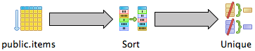
EXPLAIN (ANALYZE, VERBOSE) SELECT DISTINCT n FROM items;

Unique  (cost=131666.34..136666.34 rows=498824 width=4) (actual time=766.775..1229.040 rows=631846 loops=1)
  Output: n
  ->  Sort  (cost=131666.34..134166.34 rows=1000000 width=4) (actual time=766.774..1075.712 rows=1000000 loops=1)
        Output: n
        Sort Key: items.n
        Sort Method: external merge  Disk: 13632kB
        ->  Seq Scan on public.items  (cost=0.00..18334.00 rows=1000000 width=4) (actual time=0.006..178.153 rows=1000000 loops=1)
              Output: n
Without more work_mem or external data structures like an index PostgreSQL merge-sorts the table between memory and disk and then iterates through the results removing duplicates, much like the classic Unix combination sort | uniq.
Sorting takes most the query time, especially if we select the string column s rather than the integer column n. In both cases the unique filter goes at about the same speed.
Custom aggregate
Thomas Vondra created a custom aggregate for counting distinct values in columns of fixed-width types (additionally the types must have at most 64 bits). Without any extra work memory or indices it beats the default sort-based counting. To install
- Clone the project, tvondra/count_distinct
- Run
make install - In your database:
CREATE EXTENSION count_distinct;
Thomas explains how the aggregate works in this blog post but the short description is that it builds a sorted array of unique elements in memory, compacting as it goes.
echo "SELECT COUNT_DISTINCT(n) FROM items;" | pgbench -d count -t 50 -P 1 -f -
# average  434.726 ms
# stddev    19.955 ms
This beats the standard count distinct aggregate which took an average of 742 ms for our dataset. Note that custom extensions written in C like count_distinct are not bound by the value of work_mem. The array constructed in this extension can exceed your memory expectations.
HashAggregate
When all rows to be counted can fit in work_mem then PostgreSQL uses a hash table to get distinct values:

SET work_mem='1GB';

EXPLAIN SELECT DISTINCT n FROM items;

HashAggregate  (cost=20834.00..25822.24 rows=498824 width=4)
  Group Key: n
  ->  Seq Scan on items  (cost=0.00..18334.00 rows=1000000 width=4)
This is the fastest way discussed thus far to get distinct values. It takes an average of 372 ms for n and 23 seconds for s. The queries select distinct n and select count(distinct n) take roughly the same amount of time to run, suggesting that the count distinct aggregate is using a HashAggregate inside as well.
Be careful, setting a high enough memory allowance to activate this method may not be desirable. Remember that work_mem applies for all concurrent queries individually, so it can add up. Besides, we can do better.
Index-Only Scan
PostgreSQL 9.2 introduced this performance feature. When an index contains all information required by a query, the database can walk through the index alone without touching any of the regular table storage ("the heap"). The index type must support index-only scans. Btree indexes always do. GiST and SP-GiST indexes support index-only scans for some operator classes but not others.
We'll use btree indices and will create one each for the n and s columns:
CREATE INDEX items_n_idx ON items USING btree (n);
CREATE INDEX items_s_idx ON items USING btree (s);
Selecting distinct values of these columns now uses a new strategy:
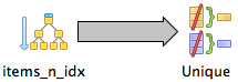
EXPLAIN SELECT DISTINCT n FROM items;

Unique  (cost=0.42..28480.42 rows=491891 width=4)
  ->  Index Only Scan using items_n_idx on items  (cost=0.42..25980.42 rows=1000000 width=4)
But now we come to a quirk, SELECT COUNT(DISTINCT n) FROM items will not use the index even though SELECT DISTINCT n does. As many blog posts mention ("one weird trick to make postgres 50x faster!") you can guide the planner by rewriting count distinct as the count of a subquery:
-- SELECT COUNT(DISTINCT n) FROM items;
-- must be rewritten as
EXPLAIN SELECT COUNT(*)
  FROM (SELECT DISTINCT n FROM items) t;

Aggregate  (cost=34629.06..34629.07 rows=1 width=0)
  ->  Unique  (cost=0.42..28480.42 rows=491891 width=4)
        ->  Index Only Scan using items_n_idx on items  (cost=0.42..25980.42 rows=1000000 width=4)
An in-order binary tree traversal is fast. This query takes an average of 177 ms (or 270 ms for the s column).
A word of warning. When work_mem is high enough to hold the whole relation PostgreSQL will choose HashAggregate even when an index exists. Paradoxically, giving the database more memory resources can lead to a worse plan. You can force the index-only scan by setting SET
enable_hashagg=false; but remember to set it true again afterward or other query plans will get messed up.
Estimated Counts
HyperLogLog
The previous techniques rely on either fitting an index, hash-table or sorted array in memory, or else consulting the statistics tables from a single database instance. When data grows truly large and/or spreads between multiple database instances these techniques begin to break down.
Probabilistic data structures help here, they give fast approximate answers and easily parallelize. We'll use one for querying distinct counts, a cardinality estimator called HyperLogLog (HLL). It uses a small amount of memory to represent a set of items. Importantly for us its union operation is lossless, meaning taking the union of arbitrary HLL values does not degrade the precision of their estimation.
The intuitive idea behind HLL is rooted in the behavior of a good hash function, particularly the distance between hashed values. A function which distributes items evenly tends to keep them spread apart. As more items are hashed they begin to run out of room and crowd closer together. By keeping track of some of the smallest distances between hashed values the algorithm can estimate the most likely number of hashed inputs that caused the crowding.
Let's measure the speed. First install the PostgreSQL extension.
- Clone postgresql-hll
- Run
make install - In your database:
CREATE EXTENSION hll;
The way it plays out is by providing a fast aggregate that acts on a sequential scan:
EXPLAIN SELECT #hll_add_agg(hll_hash_integer(n)) FROM items;

Aggregate  (cost=23334.00..23334.01 rows=1 width=4)
  ->  Seq Scan on items  (cost=0.00..18334.00 rows=1000000 width=4)
The average speed of HLL count distinct on n is 239 ms, and 284 ms on s. Thus it is slightly slower than an index-only scan for data of this size. Its true strength comes from the fact that HLL unions are lossless, associative and commutative. This means they can be parallelized across servers and combined for a final result.
Parallelization
Applications that conduct real-time analytics, such as google analytics, use counts extensively and counting is an operation which can parallelize well. This section will measure the performance of a few techniques in a small Citus cluster running on Citus Cloud.
The general idea is to run separate database instances (workers) across multiple machines. The instances share a schema and each instance holds portions (shards), of the total dataset. Workers can count rows in parallel.
Setting up a Cluster
For our example we will create a small cluster, as our purpose is to compare the performance improvements of several techniques rather than strive for ultimate benchmarking speed.
For this example I created an eight-machine cluster on Citus Cloud and selected the smallest allowable hardware configuration for each worker. If you would like to try this example yourself you can sign up for an account.
After creating a cluster I connect to the coordinator node to run the SQL. First create a table as before.
CREATE TABLE items (
  n integer,
  s text
);
At this point the table exists only in the coordinator database. We need to shard the table across the workers and then populate the shards with rows. Citus assigns each row to a unique shard by looking at the values in our choice of "distribution column." Below we tell it to distribute future rows in the items table by hashing their n column to a shard assignment.
SELECT master_create_distributed_table('items', 'n', 'hash');
SELECT master_create_worker_shards('items', 32, 1);
We'll load random data into the shards through the coordinator node. (Citus also supports MX, a "masterless" mode for faster data loading but we don't need it for this example).
After obtaining the cluster coordinator database URL, run the following on a computer with fast network access. (All the generated data passes through this computer, hence the need for good network speed.)
cat << EOF > randgen.sql
COPY (
    SELECT
      (random()*100000000)::integer AS n,
      md5(random()::text) AS s
    FROM
      generate_series(1,100000000)
  ) TO STDOUT;
EOF

psql $CITUS_URL -q -f randgen.sql | \
psql $CITUS_URL -c "COPY items (n, s) FROM STDIN"
Whereas we used a million rows in the single-database tests, this time we turned it up to a hundred million.
Exact Counts
Non-Distinct
Plain counts (non-distinct) have no problems. The coordinator runs the query on all workers and then adds up the results. The output of EXPLAIN shows the plan chosen on a representative worker ("Distributed Query") and the plan used on the coordinator ("Master Query").
EXPLAIN VERBOSE SELECT count(*) FROM items;

Distributed Query into pg_merge_job_0003
  Executor: Real-Time
  Task Count: 32
  Tasks Shown: One of 32
  ->  Task
        Node: host=*** port=5432 dbname=citus
        ->  Aggregate  (cost=65159.34..65159.35 rows=1 width=0)
              Output: count(*)
              ->  Seq Scan on public.items_102009 items  (cost=0.00..57340.27 rows=3127627 width=0)
                    Output: n, s
Master Query
  ->  Aggregate  (cost=0.00..0.02 rows=1 width=0)
        Output: (sum(intermediate_column_3_0))::bigint
        ->  Seq Scan on pg_temp_2.pg_merge_job_0003  (cost=0.00..0.00 rows=0 width=0)
              Output: intermediate_column_3_0
For reference the count query completes in an average of 1.2 seconds on this cluster. Distinct counts pose a more difficult problem across shards.
Distinct
The difficulty with counting distinct values of a column across shards is that items may be duplicated between shards and thus double-counted. However this is not a problem when counting values in the distribution column. Any two rows with the same value in this column will have been hashed to the same shard placement and will avoid cross-shard duplication.
For count distinct on the distribution column Citus knows to push the query down to each worker, then sum the results. On our example cluster it completes in an average of 3.4 seconds.
The more difficult case is doing a distinct count of a non-distribution column. Logically there are two possibilities:
- Pull all rows to the coordinator and count there.
- Reshuffle rows between workers to avoid duplication of column values between workers, then do a distinct count on each worker and sum the results on the coordinator.
The first option is really no better than counting on a single database instance -- in fact it is exactly that, plus high network overhead. The second option is the way to go.
The second option is called "repartitioning." The idea is to make temporary tables on the workers using a new distribution column. Workers send rows amongst each other to populate the temp tables, perform the query, and remove the tables. Different distributed databases perform repartitions under different query conditions. The specific details of repartition queries in Citus are beyond the scope of this article.
Estimated Count Distinct
Cardinality estimators like HLL are a lifesaver in distributed databases. They allow the system to make distinct counts for even non-distribution columns with little network overhead: the HLL datatype has a small byte size and can be sent quickly from workers to the coordinator. Because its union operation is lossless we needn't worry about the number of workers affecting its precision.
On Citus in particular you don't need to explicitly invoke postgresql-hll functions. Simply make citus.count_distinct_error_rate non-zero and Citus will rewrite count distinct query plans to use HLL. For instance:
SET citus.count_distinct_error_rate = 0.005;
EXPLAIN VERBOSE SELECT count(DISTINCT n) FROM items;

Distributed Query into pg_merge_job_0090
  Executor: Real-Time
  Task Count: 32
  Tasks Shown: One of 32
  ->  Task
        Node: host=*** port=5432 dbname=citus
        ->  Aggregate  (cost=72978.41..72978.42 rows=1 width=4)
              Output: hll_add_agg(hll_hash_integer(n, 0), 15)
              ->  Seq Scan on public.items_102009 items  (cost=0.00..57340.27 rows=3127627 width=4)
                    Output: n, s
Master Query
  ->  Aggregate  (cost=0.00..0.02 rows=1 width=0)
        Output: (hll_cardinality(hll_union_agg(intermediate_column_90_0)))::bigint
        ->  Seq Scan on pg_temp_2.pg_merge_job_0090  (cost=0.00..0.00 rows=0 width=0)
              Output: intermediate_column_90_0
It's fast too: 3.2 seconds for counting distinct values of n, and 3.8 seconds for s across 100 million records, on a non-distribution column and a string to boot. HLL is a great way to horizontally scale distinct count estimates in a distributed database.
Reference of Techniques
| Technique | Time/1M rows | Exact | Filterable | Distinct |
|---|---|---|---|---|
| PG Stats | 0.3ms | ❌ | ❌ | ❌ |
| Parse EXPLAIN | 0.3ms | ❌ | ✅ | ❌ |
| Tally | 2ms (but slow inserts) | ✅ | ❌ | ❌ |
| count(*) | 85ms | ✅ | ✅ | ❌ |
| count(1) | 99ms | ✅ | ✅ | ❌ |
| Idx Only Scan | 177ms | ✅ | ✅ | ✅ |
| HLL | 239ms | ❌ | ✅ | ✅ |
| HashAgg | 372ms | ✅ | ✅ | ✅ |
| Custom Agg | 435ms (64-bit col) | ✅ | ✅ | ✅ |
| Mergesort | 742ms | ✅ | ✅ | ✅ |
HyperLogLog (HLL), although losing slightly to index-only scans in a single database on a table of one million rows, shines in larger tables (> 100GB). It is also particularly good in a distributed database, allowing real-time distinct count estimation over enormous datasets.
We hope you found this guide on methods of counting in PostgreSQL helpful. If you have any questions about this post, or about how to effectively count over very large datasets please feel free to join us in our Citus Public Slack channel to chat.
Updated Nov 2020: And finally, if you did find this post useful and want to stay connected to our latest blog posts on Postgres and Citus, you can also follow us on Twitter @citusdata, or sign up for our Citus monthly technical newsletter (below.)